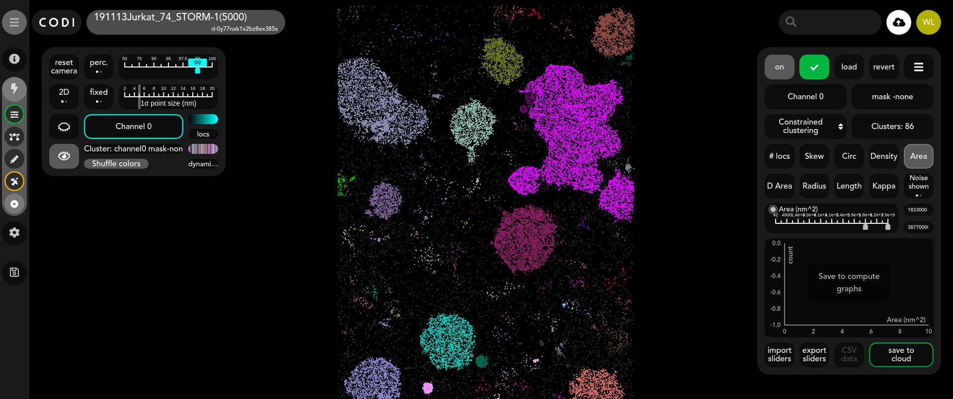
Tool view

Purpose of tool

Contents

• Running the tool

• Inspecting outputs

  • Viewing results

  • Inspecting analysis results

• Optional: Refinement of clustering results

  • Constrained clustering

  • DBSCAN*

• Exporting results

  • Saving raw cluster data

  • Saving histograms

Running the tool

Clustering can be run with default parameters by clicking “run” in the widget. This will apply any pre-processing steps loaded in the workflow to the localisations before clustering each channel individually. For more fine-grained control, a menu can be accessed by clicking the three horizontal line icon to reveal further options.

For multi-channel datasets, it is possible to select which channels to cluster as well as whether to cluster them together (when “Merged” is highlighted) or separately.

The following HDBSCAN parameters can also be selected before clustering:

• Minimum samples (Min samples)

  • This is related to the minimum density of the clusters

• Minimum number of localisations per cluster (Min size)

  • This sets a lower limit on the size of a cluster

Previous clustering executions can also be selected using the load button. Once a clustering execution has finished it should automatically load in the clustering results from the first ROI and channel (if multiple are present, the user can toggle between them).

Current and previous clustering executions can also be viewed and selected by clicking on the load button.

Inspecting outputs

Once the results are loaded, a new layer is added for the clusters as shown below. Each cluster is shown in a different colour by default, the “Shuffle colors” button randomly reorders these colors.

There is also the option to show or hide noise points in the visualisation. These are points that the algorithm has not placed inside a cluster.

Only one channel-mask combination can be viewed at once.

Cluster features

From this widget the user can inspect the distribution of each cluster feature, toggle between the different ROIs and channels, refine the clusters and export the data. The widget also displays the total number of clusters found.

The following cluster features are calculated:

• Number of localisations

• Skew - The ratio of the major to the minor axis

• Circularity - A measure where 1 corresponds to a circle, and lower values are assigned to more irregularly shaped clusters

• Density - Number of localisations in a cluster divided by the area of the cluster

• Area - Computed from the convex hull of the cluster

• Discretised area - A measure of a cluster’s area based on binning its localisations into pixels

• Radius of gyration

• Length - An approximation of the longest axis

• Kappa - model parameter relating to the least dense parts of a cluster.

More details are available in the technical document on clustering.

Refinement of clustering results

Clustering methods rely on statistical measures to detect features in an image. However, the features of interest for a particular biological analysis may not be the most statistically significant and thus not found by the initial clustering. For example, it is possible that the structures of interest in the image are circular but the clustering algorithm will not, by default, look for circular clusters. In such situations, constraining the clusters based on geometric/morphological features can be useful. The clustering tool enables this by providing two further tools for further refinement of clusters.

• Constrained clustering

  • This approach allows the user to set constraints on the cluster properties and then recluster the data according to these constraints.

• DBSCAN*

  • This approach is similar to DBSCAN but allows for real time adjustment of the eps parameter to choose a cluster length scale.

NOTE: The graphs disappear when the refinement process is started. The original clustering results are still available from the “Load” menu, and the “revert” button will undo any changes. Once the refinement is complete, click “save to cloud” to compute the new feature distribution graphs and/or to use the clusters for a subsequent step in the workflow.

Constrained clustering

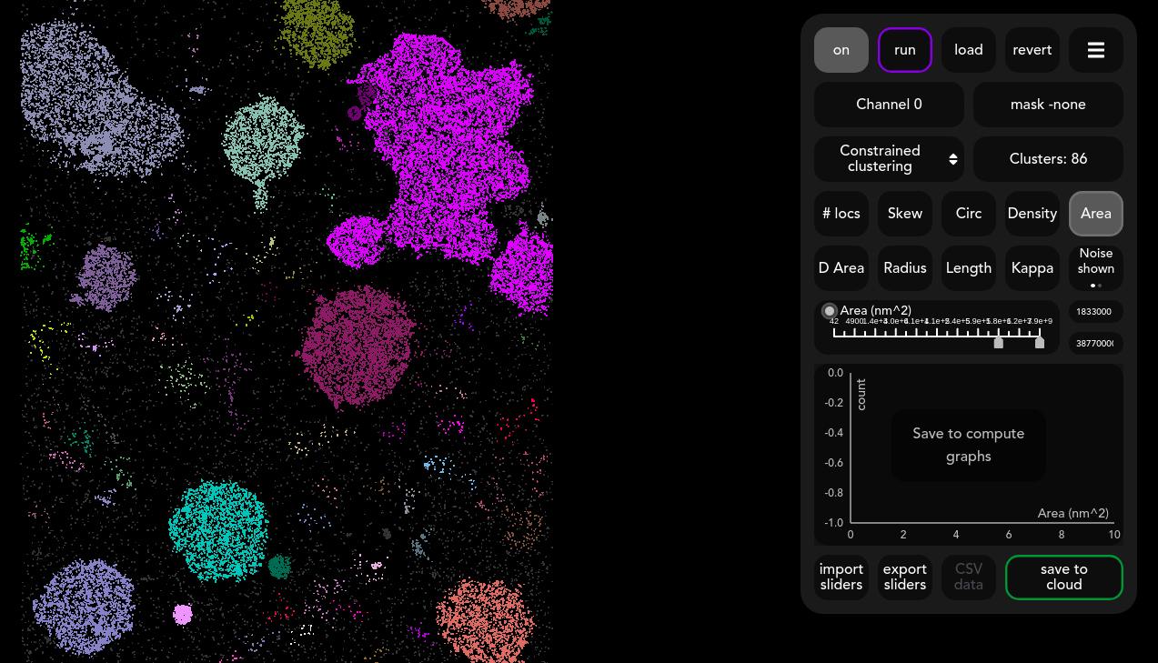
For each feature, the sliders can be adjusted to restrict the type of clusters being computed. The algorithm will then dynamically recluster the localisations to fit these constraints. In this case, a minimum area threshold has been selected, which has caused smaller clusters to coalesce into larger ones. Multiple constraints can be selected, and a grey outline is shown around those that are active. A quick way to see the effect of an adjusted constraint is to click the toggle on the slider on/off for that feature.

The slider ticks have been selected such that it should be easy to choose the right constraints but it is also possible to input specific numbers by hand in the text boxes on the right of the slider.

DBSCAN*

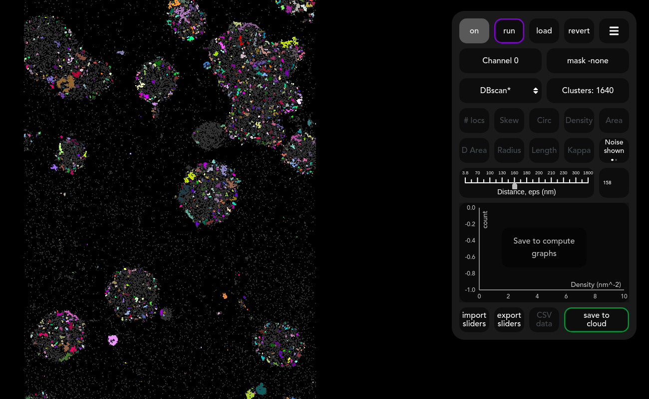
An alternative to constrained clustering is to use DBSCAN*. This refinement method only has one slider ‘Distance’ which mimics the behaviour of the DBSCAN eps parameter (more info). Move this slider to change the length scale of the clusters. The effect of the increasing the slider can be seen in the image below.

Larger values of eps allows for a larger separation of points within each cluster, which typically leads to less dense and larger clusters.

Exporting results

Saving raw cluster data

The “CSV data” button provides a CSV where each row corresponds to an individual cluster. The CSV contains the ID of each cluster, as well as each cluster feature.

Saving histograms

Each of the histograms can be downloaded as an image or the raw data can also be downloaded as a CSV. Use the download button in the top right corner of the graph.

An example of the CSV file for the skew histogram is given below: