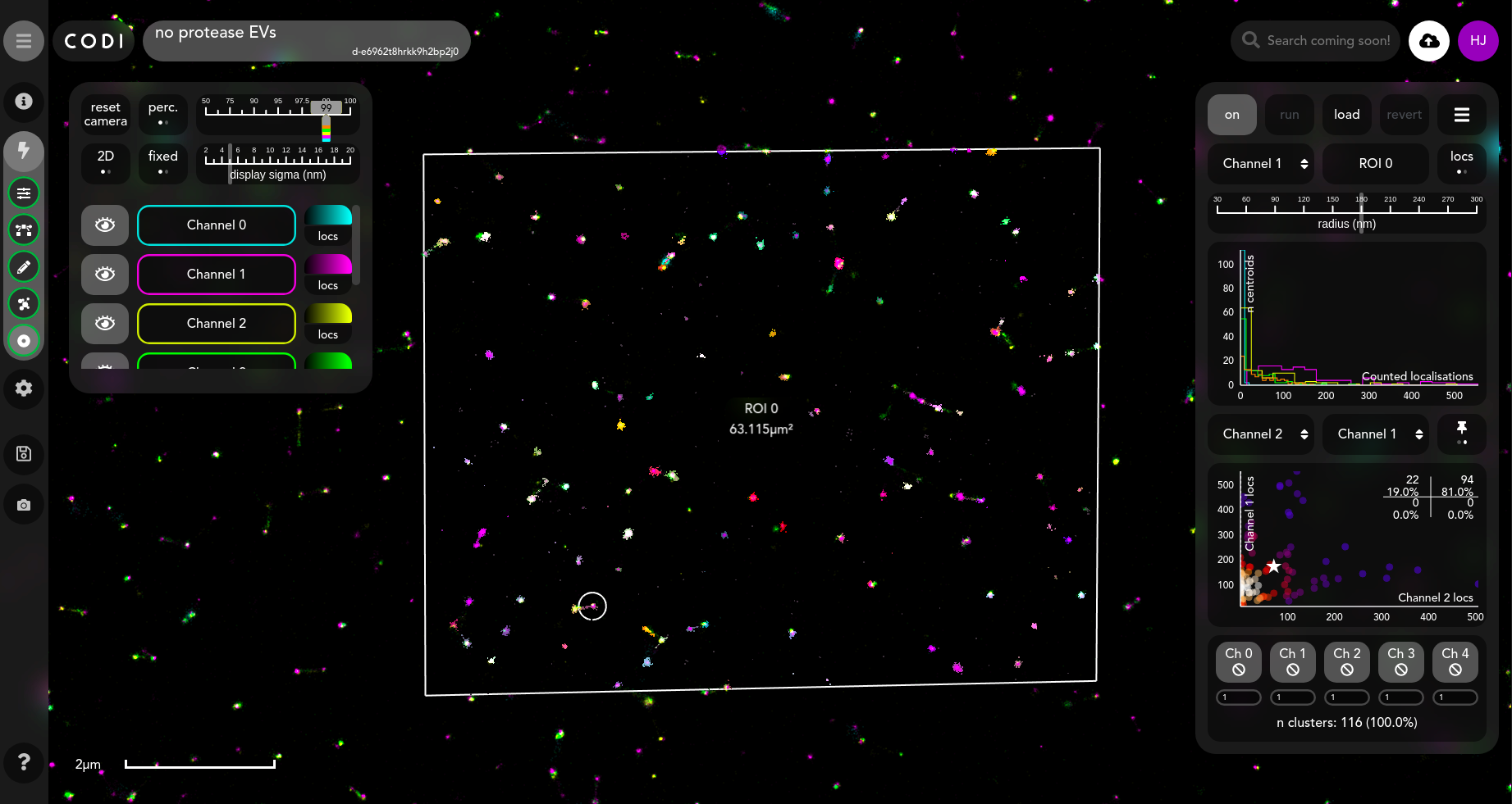
Tool view

Purpose of tool

Contents

• Inputs

• Results

• Outputs

Inputs

The centre points for counting come from a loaded clustering execution. A clustering execution must be loaded and have a green ring around it in the workflow sidebar.

 

The following parameters have defaults but can also be adjusted by the user:

• Max radius: The radius around the centre point inside which the localisations or bins are counted

• N rings: The number of circle sizes up to the max radius for which should be precomputed

• Bin size: This allows the user to choose the size of the bins when the counting is done on number of spatial bins containing localisations, as opposed to just localisations

• Count threshold: This allows the user to define the number of localisations that a bin must have for it to be counted

• Import/export config: Loads in a previous set of parameters used for the counting tool

There are additional optional pre-processing steps which must be loaded into the execution workflow visible on the left of the screen:

• Localisation filters

• Drift correction

• ROI selection

 

When a pre-processing result is loaded, a green ring will appear around the icon, as is shown in the example below where a localisation filtering result has been loaded for use as pre-processing step in the counting tool.

Results

Results should automatically load once the execution has completed. Previously run executions can be selected from the ‘Load’ dropdown once they have completed.

 

Localisation results

• The default results view shows localisation counting around the centre points (clustering execution centroids).

• The graph shown in the right panel is a histogram containing the number of localisations around a centre point.

• The channel being viewed is shown in the top row of the right panel.

• The radius value being considered is shown in the adjustable slider bar

• The bottom rows with the channel buttons allow the user to set thresholds for the number of localisations in a given cluster. This can be useful for finding biological objects that are positive or negative in a particular biomarker.

• On the back of the panel, there is an import config and export config option, which allows the user to import/export the parameters of the counting tool
  

Binned results

In the top right of the menu the counting tool can be toggled into bins mode. Using this option, the localisations are discretised into a pixel grid for each centre point, and a threshold is taken on the counts in each bin. Bins which meet the threshold are counted, giving an area metric for each channel around each centre point.

Interacting with results

The search radius can be adjusted up to, and including, the set maximum search radius, and the plots will update interactively to show the effects of this adjustment.

 

The scatter plot is also interactive; the default mode is for selection of scatter points, which each correspond to a centre point somewhere in the field of view. Here, a selected point is marked with a star in the scatter plot, and its selection has zoomed the viewer to the corresponding centre point, marked with a white circle. Users can also select clusters in the viewer to highlight their counting circle and corresponding point on the scatter plot.

 

When the channels in the bottom two rows are clicked, the scatter plot switches to gated analysis mode, which allows the user to look at specific regions in the graph. The ranges entered in the boxes adjacent to the channels define the ranges on the number of localisations/bins counted from a channel within a radius of a centre point, in order for that centre point to be called “positive” for that channel. As the centre points in this tool represent cluster centroids, the counts around these points gives an estimate of how much of a molecule is in the vicinity of a given cluster.

The pair of channels being examined in the plots can be changed by selecting the dropdowns above the scatter plot.

Outputs

Both .png and .svg image files of the two plots can be downloaded by hovering over them and clicking the download button. CSV data relating to the positivity/negativity of the analysis, using the gating as thresholds, is also available from the scatter plot.